COMP 320

（我也不知道为什么要做 COMP 320 的 Notes，这感觉就像在我这个年纪学习如何上厕所）

Repoducibility

Each process owns address space. (one huge list)
Multiple lists start at different address in address space; normally, append is faster than pop, since pop need to move all next items forward 4 bytes. (? Really)
Use ASCII to store strings, use specific ISA to store codes.
A CPU can only run programs that use instructions it understands, interpreters/compiler make it sense to run the same code on different machines.
OS: allocate and abstract resources
commits: explicit snapshots/checkpoints; explicit commit messages (who, what, when, why)
Tag “good” commits to create releases.
git:
8.1 HEAD: wherever you currently are (one and only one)
8.2 tag: label tied to a specific commit number
8.3 branch: label tied to end of chain (moves upon new commits)
8.4 detached HEAD: refers to a situation where the HEAD pointer (which usually points to a branch reference) directly points to a specific commit, rather than pointing to the latest commit of a branch. In simpler terms, when you’re working in a normal branch (say, “master” or “main”), the HEAD points to the name of that branch, and that branch name points to the latest commit. Any new commits you make will advance the branch to point to the newer commit, and HEAD follows along because it’s pointing to the branch name.
time.time() returns seconds since 1970

Performance

Affect performance
1.1: Speed of CPU
1.2: Speed of Interpretation
1.3: Algorithm
1.4: Input size
Complexity analysis only cares about “big” inputs.
A step is any unit of work with boudned execution time. (“bounded” does not mean “fixed”)
Big O:
4.1 Goal: categorize functions by how fast they grow. Do not care about scale. Do not care about small inputs. Care about shape of the curve. Find some multiple of a general function that is an upper bound
O(1): x = L[0], x = len(L), L.append(x), L.pop(-1)
O(N): L.insert(0, x), L.pop(0), x = max(L), L2.extend(L1), x = sum(L), found = X in L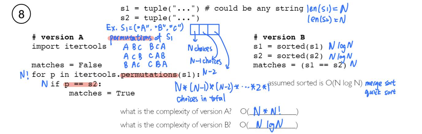

Object Oriented Programming

Dog.speak(fido, 5), not an example of type-based dispatch.
Special Methods: (implicity)
2.1 Not all __some__ is special methods
2.2 __str__, __repr__, control how an object looks when we print it or see it in Out[N].
2.3 __repr_html__, generate HTML to create more visual representaitons of objects in Jupyter.
2.5 __eq__, __lt__, define how == behaves for two different objects, sorting(__lt__)
2.6 __len__, __getitem__, build our own sequences that we index, slice, and loop over.
2.7 __enter__, __exit__, context managers, (like automatically close file)
Inheritance: method inheritance, method resolution order, overriding methods, constructor, calling overidden methods, abstrace base classes
Every class in python implicitly inherits from the build-in object class if no other explicitly specified.

Web

WebDriver.get(u) loads the web page with URL. WebDriver.find_element(a, b) returns the first WebElement which has attribute a being b. WebDriver.find_elements(a, b) returns a list of WebElements. a can be id: unique, name: mulitple elements can have the same name, tag name: by its tag. Get all the links element: driver.find_elements("tag name", "a"), tanle 是 table 不是 td, 获取 link 以后获得内部的 attibute, .get_attribute("attribute_name")
Send value to a variable text as input, text.send_keys("2023)
ol, ul, ordered or unordered list, select, drop-down list
Tables can be scraped by find_element("tag name", "table") and iterate over find_elements("tag name", "tr") and find_elements("tag name", "td")
ith cell of j th row? element.find_elements("tag name", "tr")[i - 1].find_elements("tag name", "td")[j - 1].text. 第一个元素可以忽略 index
对于已经获得的element, 通过.attribute访问内部元素，对于text内容, element.text,比如 <a href="page.html" target="_blank">link<\a> 获取link, elememt.clear清空
for static pages (without JavaScript modifications), pandas.read_html can return a list of DataFrames, one for each table, on the web page.
WebDriver.save_screenshot("file.png) saves a screenshot of the web page to a file with name file.png. Firefox has the option to take screenshot of the full page using WebDriver.save_full_screenshot("file.png"). a screenshot of a specific element can be save using WebElement.screenshot("file.png").
Polling:
1. Use time.sleep(s) to wait s seconds, and use it inside a while loop to wait for an event to happen, before accessing or interacting with the updated elements.
2. Avoid infinite loop.
3. selenium.webdriver.support has implicit and explicit waits, so that the driver keeps polling until a certain condition is met or a certain time has passed.
Robots Exclusion:
1. Some websites disallow web crawling. The rules are specified in a robots.txt.
2. urllib.robotparser can be used to check whether a website allows scraping
3. RobotFileParser.can_fetch(useragent, url) returns True if the useragent (for example, “*“) is allowed to fetch url
Access Links:
1. WebDriver.find_elements("tag_name", "a") finds all the hyperlinks on the page.
2. Use url = WebElement.get_attribute("href") to get the URL of the hyperlink, then use WebDriver.get(url) to load that page.
Infinite Graph Search:
1. If the pages are nodes, and links on one page to another page are edges, the digraph formed by pages will possibly have infinite depth and may contain cycles.
2. To find a specific (goal) page, or to discover reachable pages from the initial page, breadth first search should be used (since depth first search may not terminate on trees with infinite depth).
3. Since there are cycles, a list of visited pages should be kept.
Search Heuristics:
1. Searching the nodes in the order according to the heuristic is called best first greedy search. (GBS) 取 h 最小
2. A search, estimate of how close the current node is to the goal in the search tree. the current distance from the initial node plus the heuristic
3. A heuristic that always underestimates the true distance is called an admissible heuristic. A*
Priority Queue:
1. For GBS search, use a Priority Queue with the priority based on the heuristic.
2. For A search, use a Priority Queue with the priority based on current distance plus the heuristic.
Give an example of a goal node that is reachable (finite edges away) from the initial node, but the following method cannot find the goal node. Assume the nodes are ${G, 0, 1, 2, …}$ where 0 is the initial node and is the goal node, and each node has finite number of children.
BFS, A: impossible, 必定可以找到
DFS，GBS：优先度高的那各分支无穷远
Flask:
1. Flask is a simpler web framework of Django. Django is a more popular package.
2. Flask will be used to create or modify web pages. It can be useful for collecting visitor data when interacting with the web pages and displaying them on the web pages.
3. app = flask.Flask(...), root url: @app.route("/"), other: @app.route("/abc"), run: app.run(host="0.0.0.0", debug=False, threaded=False)
4. Binding functions:
  1
  2
  3
  @app.route("/index") def index() return "Hello World!"
  binds the index function to the page IP address/index, meaning it will display a web page that says “Hello World”. “Hello World” can be replaced by any text or HTML string. HTML string can be read from existing HTML files then modified. It can also be generated by packages such as pandas. pandas.read_csv("data.csv").to_html()
Process query string inside a flask application: flask.request.args
Binding Multiple Path:
1. To bind multiple paths, variable rules can be added, @app.route("/index/<x>") def index(x) return f"Hello {x}" will display a web page that says “Hello World” when the path IP address/index/World is used.
2. <int:x> for int, <float:x> for float, <path:x> for string but allows /
Redirectling Pages:
1. return flask.redirect(url) redirects the current path to another with URL url
2. return flask.redirect(flask.url_for("index")) redirects the current path to another which binds to the function index()
3. return flask.redirect(flask.url_for("index", x = "World")) redirects the current path to another which binds to the function index("World")
Collecting Vistor Information:
1. flask.request.remote_addr can be used to find the remote IP address of the visitor -> sercive provider, location
2. flask.request.user_agent.string can be used to find the user agent of the visitor. -> browser, os, device information
Rate Limiting:
1. Prevent web scraping, 429, Too Many Requests
2. In this case, the visitor’s IP address and visit time can be stored in a list: in case the next visit time is too close to the previous one, the visitor can be redirected to another page, or more commonly, responded with a error message, for example, return flask.Response("...", status = 429, headers = {"Retry-After": "60"}) tells the visitor to retry after 60 seconds.
3. 100s: Informational, 200s: Successful, 300s: Redirection, 400s: Client Error, 500s: Server Error 200: OK, 304: Not Modified, 400: Bad Request, 401: Unauthorized, 404: Not Found, 409: Conflict, 413: Request Entity Too Large, 500: Internal Server Error， 405：Method not allowed(比如尝试 get 只允许 Put 的), 501: Not implemented(没有这个函数)
AB Testing:
1. Two or more versions of the same page can be displayed to the visitor randomly to compare which one is better. The two versions are called control (version A) and treatment (version B) in statistics.
2. The comparison is often based on click-through rates (CTR), metric, which is computed as the number of clicks on a specific link on the page divided by the number of times the page is displayed to the visitor.
3. CTR is also used for advertisement, computed as the number of clicks on the ad divided by the number of times the ad is shown to the visitor.
4. Having a large sample size will have small p-value.
5. When introduce a new version “B”, might be terrible but still want to evaluate it, start with “0” of B, then slowly increase
6. fisher_exact() 算出来的，大于 thresold 就两者没有显著差异
Displaying Pages:
1. The choice of which page to display can be random, for example, if random.random() < 0.5: return "Version A" else return "Version B"
2. It can also be displayed in a fixed ordering, for example, suppose count is a global variable to keep track of the number of visitors, then if count % 2 == 0: return "Version A" else return "Version B" count = count + 1 would alternate between the two versions.
Tracking Visitors:
1. IP address or user agent information can be used to figure out which version of the page is displayed to which visitors
2. Cookies can be used too, use flask.request.cookies.get(key, default) to get a cookie (and returns default if no such cookies exist), and flask.Response.set_cookie(key, value) to set a cookie. Cookies are stored on the visitors’ computer as text files.
3. Query strings can be used to figure out which version of a page the visitor came from, it is the string after “?” at the end of a URL
Query Strings:
1. "index?x=1&y=2" is a URL specifying the path “index” with the query string x=1 and y=2. Use flask.request.args to get a dictionary of key-value pairs of the query string.
2. To perform AB testing of a page with two versions, both contain a link to index: on version A, the URL can be <a href="index?from=A">Link<\a>, and on version B, the same URL can be <a href="index?from=B">Link<\a>. If version A URL is used, request.args["from"] would be “A” and if version B URL is used request.args["from"] would be “B”
Two Armed Bandit Example: The pages represented by boxes have fixed but possibly different average values between 0 and 1. Click on one of them to view a random realization of the value from the box (i.e. a random number from a distribution with the fixed average). The goal is to maximize the total value (or minimize the regret) given a fixed number of clicks. Which box has the largest mean reward? 类似于大数定理，经验平均数在 N 无穷大的时候趋近于真实平均
Multi-Armed Bandit:
1. This design can lead to a large “regret”, for example, if displaying bad version is costly. In other settings such as drug or vaccine trials and stock selection, experimenting with bad alternatives can be costly.
2. The problem of optimal experimentation vs exploitation is studied in reinforcement learning as the multi-armed bandit problem
Upper Confidence Bound:
1. a no-regret algorithm that minimizes the loss from experimentation
2. After every version is displayed once, the algorithm keeps track of the average value (for example click-through rate) from each version, say $\hat{\mu}{A}$, $\hat{\mu}{B}$ and computes the UCBs $\hat{\mu}{A} + c\sqrt{\frac{2log(n)}{n{A}}}$ and $\hat{\mu}{B} + c\sqrt{\frac{2log(n)}{n{B}}}$, where $n$ is the total number of visitors, $n_{A}$ is the number of visitors of version A, $n_{B}$ is the number of visitors of version B, and $c$ is a constant, and always picks the version with a higher UCB.
Live Plots on Flask Sites:
1. A function that returns an image response can be used for @app.route("/plot.png") or @app.route("/plot.svg"). SVG: Scalable Vector Graphics, represented by a list of geometric shapes such as points, lines, curves
2. An image response can be created using flask.Response(image, headers={"Content-Type": "image/png"}) or flask.Response(image, headers={"Content-Type": "image/svg+xml"}), where the image is a bytes object and can be obtained using io.BytesIO.getvalue() where io.BytesIO creates a “fake” file to store the image.
3. On the web page, display the image as <img src="plot.png"> or <img src="plot.svg">
Plotting Low Dimensional Data Sets:
1. One to three dimensional data items can be directly plotted as points (positions) in a 2D or 3D plot.
2. For data items with more than three dimensions (“dimensions” will be called “features” in machine learning), visualizing them effectively could help with exploring patterns in the dataset. Summary statistics such as mean, variance, covariance etc might not be sufficient to find patterns in the dataset.
3. For item dimensions that are discrete (categorical), plotting them as positions may not be ideal since positions imply ordering, and the categories may not have an ordering.

Encoding	Continuous	Ordinal 顺序？	Discrete (Categorical)
Position	Yes	Yes	Yes
Size	Yes	Yes	No
Shape	No	No	Yes
Value	Yes	Yes	No
Color	No	No	Yes
Orientation	Yes	Yes	Yes
Texture	No	No	Yes

Seaborn plots:
1. one of the data visualization libraries that can make plots for exploring the datasets with a few dimension.
2. Suppose the columns are indexed by $c1, c2, …$, then seaborn.relplot(data = ..., x = "c1", y = "c2", hue = "c3", size = "c4", style = "c5"visualizes the relationship between the columns by encoding c1 by x-position, c2 by y-position, c3 by color hue if the feature is discrete, and by color value if it is continuous, c4 by size, c5 by shape (for example, o’s and x’s for points, solid and dotted for lines) if the feature is discrete.
Multiple Plots of Seaborn:
1. For discrete dimensions with a small numbers of categories, multiple plots can be made, one for each category.
2. seaborn.relplot(data = ..., ..., col = "c6", row = "c7") produces multiple columns of plots one for each category of c6, and multiple rows of plots one for each category of c7.
3. seaborn.pairplot produces a scatter plot for each pair of columns (features) which could be useful for exploring relationships between pairs of continuous features too. 查找两个 feature 之间的关系
4. Chernoff Face: used to display small low dimensional datasets. The shape, size, placement and orientation of eyeys, ears, mouth and nose are visual encodings.
Plotting High Dimensional Data Sets
1. To figure out the most important dimensions, which are not necessarily one of the original dimensions, unsupervised machine learning techniques can be used. 降维 PCA

Graph

Layouts:
1. Circular layout and arc (chord) layout are simple for the computer, but difficult for humans to understand the shape of the graph.
2. Force-Directed Placement (FDP) treats nodes as points and edges as springs and tries to minimize energy. It is also called spring model layout.
Tree Diagrams:
1. Trees are special graphs for which each node has one parent, and there are more ways to visualize a tree
2. Can be plotted “manully” using matplotlib
Plotting Primitives: 基本图形
1. matplotlib.patches contain primitive geometries such as Circle, Ellipse, Polygon, Rectangle, RegularPolygon and ConnectionPatch, PathPatch, FancyArrowPatch
2. matplotlib.text can be used to draw text; it can render math equations using TeX too
Plotting Graphs:
1. 画点: A node (indexed i) at $(x,y)$ can be represented by a closed shape such as a circle with radius $r$, for example, matplotlib.patches.Circle((x, y), r), and matplotlib.text(x, y, "i").
2. 画边: An edge from a node at $(x_1, y_1)$ to a node at $(x_2, y_2)$ can be represented by a path (line or curve, with or without arrow), for example, matplotlib.patches.FancyArrowPatch((x1, y1), (x2, y2)), or if the nodes are on different subplots with axes ax[0], ax[1], matplotlib.patches.ConnectionPath((x1, y1), (x2, y2), "data", axesA = ax[0], axesB = ax[1])
3. To specify the layout of a graph, a list of positions of the nodes are required (sometimes parameters for the curve of the edges need to be specified too).
Ways to Specify Curves:
1. A curve (with arrow) from $(x_1, y_1)$ to $(x_2, y_2)$ can be specified by the (1) out-angle and in-angle, (2) curvature of the curve, (3) Bezier control points
2. FancyArrowPatch((x1, y1), (x2, y2), connectionstyle=ConnectionStyle.Angle3(angleA = a, angleB = b)) plots a quadratic Bezier curve starting from $(x_1, y_1)$ going out at an angle $a$ and going in at an angle $b$ to $(x_2, y_2)$.
3. FancyArrowPatch((x1, y1), (x2, y2), connectionstyle=ConnectionStyle.Arc3(rad = r)) plots a quadratic Bezier curve from $(x_1, y_1)$ to $(x_2, y_2)$ that arcs towards a point at distance r times the length of the line from the line connecting $(x_1, y_1)$ and $(x_2, y_2)$.
Bezier Curves:
1. Beizer curves are smooth curves specified by control points that may or may not be on the curves themselves. The curve connects the first control point and the last control point. The vectors from the first control point to the second control point, and from the last control point to the second-to-last control point, are tangent vectors to the curve.
2. The curves can be constructed by recursively interpolating the line segments between the control points.
3. PathPatch(Path([(x1, y1), (x2, y2), (x3, y3)], [Path.MOVETO, Path.CURVE3, Path.CURVE3])) draws a Bezier curve from $(x_1, y_1)$ to $(x_3, y_3)$ with a control point $(x_2, y_2)$.
Coordinate Systems:
1. There are four main coordinate systems: data, axes, figure, and display
2. The primitive geometries can be specified using any of them by specifying the transform argument, for example for a figure fig and axis ax, Circle((x, y), r, transform = ax.transData), Circle((x, y), r, transform = ax.transAxes), Circle((x, y), r, transform = fig.transFigure), or Circle((x, y), r, transform = fig.dpi_scale_trans).
3. How to draw a quadratic Bezier curve with control points (0, 0), (1, 0), (1, 1)?
  This curve has the same shape as the curve drawn in the “Curve Example”: in particular, the start angle is 0 degrees (measured from the positive x-axis direction) and the end angle is 270 degrees or -90 degrees, and the distance of the line segment connecting the midpoint between (0, 0) and (1, 1) (which is (1/2, 1/2)) and the middle control point (which is (1, 0)) is half of the length of the line segment connecting (0, 0) and (1, 1), or $\sqrt{(1-\frac{1}{1})^2 + (0-\frac{1}{2})^2} = \frac{1}{2}\sqrt{(1-0)^2+(1-0)^2}$
  Therefore, use any path patch with connectionstyle ConnectionStyle.Angle3(0, -90) or ConnectionStyle.Arc3(1/2) to plot the curve.

Coordinate System	Bottom Left	Top Right	Transform
Data	based on data	based on data	`ax.transData` (default)
Axes	(0, 0)	(1, 1)	`ax.transAxes`
Figure	(0, 0)	(1, 1)	`fig.transFigure`
Display	(0, 0)	(w, h) in inches	`fig.dpi_scale_trans`

Map

Map Projections:
1. Positions on a map are usually specified by a longitude and a latitude. It is often used in Geographic Coordinate Systems (GCS)
2. They are angles in degrees specifying a position on a sphere
3. It is difficult to compute areas and distances with angles, so when plotting positions on maps, it is easier to use meters, or Coordinate Reference Systems (CRS)
Regions on Maps and Polygons
1. A region on a map can be represented by one or many polygons. A polygon is specified by a list of points connected by line segments.
2. Information about the polygons are stored in shp, shx and dbf files
GeoPandas:
1. GeoPandas package can read shape files into DataFrames and matplotlib can be used to plot them. GeoSeries can do everything a Series can do, and more
2. geopandas.read_file(...) can be used to read a zip file containing shp, shx and dbf files, and output a GeoDataFrame, which a pandas DataFrame with a column specifying the geometry of the item.
3. GeoDataFrame.plot() can be used to plot the polygons.
Conversion from GCS to CRS
1. GeoDataFrame.crs checks the coordinate system used in the data frame.
2. GeoDataFrame.to_crs("epsg:326??") or GeoDataFrame.to_crs(“epsg:326??) can be used to convert from degree-based coordinate system to meter-based coordinate system.
Creating Polygons:
1. Polygons can be created manually from the vertices using shapely too
2. Point(x, y) creates a point at $(x,y)$
3. LineString([x1, y1], [x2, y2]) or LineString(Point(x1, y1), Point(x2, y2)) creates a line from $(x_1, y_1)$ to $(x_2, y_2)$.
4. Polygon([[x1, y1], [x2, y2], ...]) or Polygon([Point(x1, y1), Point(x2, y2), ...]) creates a polygon connecting the vertices $(x_1, y_!), (x_2, y_2)$
5. box(xmin, ymin, xmax, ymax) is another way to create a rectangular Polygon
Polygon Properties:
1. Polygon.area or MultiPolygon.area computes the area of the polygon
2. Polygon.centroid computes the centroid (center) of the polygon (using meter)
3. Polygon.buffer(r) computes the geometry containing all points within a r distance from the polygon. If Point.buffer(r) is used, the resulting geometry is a circle with radius r around the point, and Point.buffer(r, cap_style = 3) is a square with “radius” r around the point
Polygon Manipulation:
1. Union and intersections of polygons are still polygons.
2. geopandas.overlay(x, y, how = "intersection") computes the polygons that is the intersection of polygons x and y, if GeoDataFrame has geometry x, GeoDataFrame.intersection(y) computes the same intersection. intersects 返回是否相交(bool), intersection 返回一个相交集合(polygon). y 可以是一个 Window, 返回指定范围内的 polygon
3. box() 返回 polygon.Ploygon 类型
4. geopandas.overlay(x, y, how = "union") computes the polygons that is the union of polygons x and y, Doc, if GeoDataFrame has geometry x, GeoDataFrame.union(y) computes the same union
5. GeoDataFrame.unary_union is the single combined MultiPolygon of all polygons in the data frame
6. GeoDataFrame.convex_hull computes the convex hull (smallest convex polygon that contains the original polygon)
Geocoding:
1. geopy provide geocoding services to convert a text address into a Point geometry that specifies the longitude and latitude of the location
2. geopandas.tools.geocode(address) returns a Point object with the coordinate for the address

Regular Expressions

Regular Expressions (Regex) is a small language for describing patterns to search for and it is used in many different programming languages
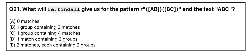
Python re package has re.findall(regex, string) and re.sub(regex, replace, string) to find and replace parts of string using the pattern regex
parentheses () are used to create capture groups. 在最后显示出来的时候会变成 tuple, 有一个括号就有一个 element，包裹嵌套括号
Raw Strings:
1. Python uses escape characters to represent special characters.
2. Raw strings r"..." starts with r and do not convert escape characters into special characters.

Code	Character	Note
`\"`	double quote	-
`\'`	single quote	-
`\\`	backslash	`"\\\""` displays `\"`
`\n`	new line	-
`\r`	carriage return	(not used often)
`\t`	tab	-
`\b`	backspace	(similar to left arrow key)

Meta Characters
+？ exactly one

Meta character	Meaning	Example	Meaning
`.`	any character except for \n	`-`	`-`
`[]`	any character inside brackets	`[abc]`	a or b or c
`[^ ]`	any character not inside brackets	`[^abc]`	not one of a, b, c
`*`	zero or more of last symbol	`a*`	zero or more a
`+`	one or more of last symbol	`a+`	one or more a
`?`	zero or one of last symbol	`a?`	zero or one a
`{ }`	exact number of last symbol	`a{3}`	exactly aaa
`{ , }`	number of last symbol in range	`a{1,3}`	a or aa or aaa
`\|`	either before or after bar	`ab\|bc`	either ab or bc
`\`	escapes next metacharacter	`\?`	literal ?
`^`	beginning of line	`^a`	begins with a
`$`	end of line	`a$`	ends with a

Shorthand
\s能都指代所有空格，包括 tab，回车

Shorthand	Meaning	Bracket Form
`\d`	digit	`[0-9]`
`\D`	not digit	`[^0-9]`
`\w`	alphanumeric character	`[a-zA-Z0-9_]`
`\W`	not alphanumeric character	`[^a-zA-Z0-9_]`
`\s`	white space	`[\t\n\f\r\p{Z}]`
`\S`	not white space	`[^\t\n\f\r\p{Z}]`

Capture Group
1. re.findall can return a list of substrings or list of tuples of substrings using capturing groups inside (...), for example, the regex ...(x)...(y)...(z)... returns a list of tuples with three elements matching x, y, z.
2. re.sub can replaces the matches by another string, the captured groups can be used in the replacement string by \g<1>, \g<2>, \g<3>, …, for example, replace ...(x)...(y)...(z)... by \g<2>\g<3>\g<1> will return yxz
Additional

Words

Supervised: use the data to figure out the relationship between the features and labels of the items, and apply the relationship to predict the label of a new item. (classification if discrete, regression if continuous)
Unsupervised: use the data to find patterns and put items into groups. (clustering if discrete, dimensionality reduction if continuous)
Feature representation: items need to be represented by vector of numbers, for categories(one-hot encoding), images and text require additional preprocessing.
Tokenization: A text document needs to be split into words. Split the string by space and punctuation, sometimes regular expression rules can be used. Remove stop words: “the”, “of”, “a”, “with”, … Stemming and lemmatization: “looks”, “looked”, “looking” to “look”. nltk has functions to do these, nltk.corpus.stopwords.words("english") to get a list of stop words in English, and nltk.stem.WordNetLemmatizer().lemmatize(word) to lemmatize the token word.
Vocabulary: A word token is an occurrence of a word. A word type is a unique word as a dictionary entry. A vocabulary is a list of word types, typically 10000 or more word types. Sometimes <s> (start of sentence), </s> (end of sentence), and <unk> (out of vocabulary words) are included in the vocabulary. A corpus is a larger collection of text. A document is a unit of text item.
Bag of words features represent documents as an unordered collection of words. Each document is represented by a row containing the number of occurrences of each word type in the vocabulary. For word type $j$ and $i$ document, the feature is $c(i,j)$, the number of times word $j$ appears in document $i$.
TF-IDF features:
1. adjust for the fact that some words appear more frequently in all documents.
2. The term frequency of word type $j$ in document $i$ is defined as $tf(i,j)=\frac{c(i,j)}{\sum_{j’}c(i,j’)}$ where $c(i,j)$ is the number of times word $j$ appears in the document $j$, and $\sum_{j’}c(i,j’)$ is the total number of words in document $i$.
3. The inverse document frequency of word type $j$ in document $i$ is defined as $idf(i,j)=log(\frac{n+1}{n(j)+1})$ where $n(j)$ is the number of documents containing word $j$, and $n$ is the total number of documents.
4. For word type $j$ and document $i$, the feature is $tf(i,j)*idf(i,j)$.
5. sklearn.feature_extraction.text.CountVectorizer can be used to convert text documents to a bag of words matrix. sklearn.feature_extraction.text.TfidfVectorizer can be used to convert text documents to a bag of words matrix

Image

Image Pixel Intensity Features: Gray scale images have pixels valued from 0 to 255 (integers, 0 being black, 255 being white), or from 0 to 1 (real values, 0 being black, 1 being white). These pixel values are called pixel intensities. The pixel value matrices can be flattened into a vector (i.e. $k$ pixel by $k$ pixel image can be written as a list of $k^2$ numbers and used as input features.
Image Preprocessing: scikit-image can be used for basic image processing tasks. skimage.io.imread (read image from file), skimage.io.imshow (show image). The images are stored as numpy.array, which can be flattened using numpy.ndarray.flatten.
Color Images:
1. RGB color images have color pixels represented by three numbers Red, Green, Blue, each valued from 0 to 255 or 0 to 1.
2. Intensity can be computed as $I = \frac{1}{3}(R+G+B)$. Other perceptual luminance-preserving conversion can be done too, $I = 0.2125R+0.7154G+0.0721B$.
3. skimage.color.rgb2gray

Convolution:

Convolution between an image and a filter (sometimes called kernel) is the dot product of every region of an image and the filter (sometimes flipped).

skimage.filters has a list of special filters.

Name	Example	Use
Identity	`[0 0 0]` `[0 1 0]` `[0 0 0]`	nothing
Gaussian	`[0.0625 0.125 0.0625]` `[0.125 0.25 0.125]` `[0.0625 0.125 0.0625]`	blur
X gradient	`[0 0 0]` `[1 0 -1]` `[0 0 0]`	vertical edges
Left (Right) Sobel	`[1 0 -1]` `[2 0 -2]` `[1 0 -1]`	vertical edges (blurred)
Y gradient	`[0 1 0]` `[0 0 0]` `[0 -1 0]`	vertical edges
Top (Bottom) Sobel	`[1 2 1]` `[0 0 0]` `[-1 -2 -1]`	vertical edges (blurred)

Image Gradient Features: One popular face recognition algorithms uses HOG (Histogram of Gradients) features.
1. Compute the X and Y gradient for each pixel (either X or Y gradient filters or Sobel filters)
2. Compute a histogram for pixel gradients in each of the 8 orientations for every 16 by 16 pixel regions (8 numbers for every 16 x 16 region)
3. Concatenate the histograms to use as the feature vector
4. skimage.feature.hog computes the HOG features

Classification

Binary Classification: For binary classification, the labels are binary, either 0 or 1, but the output of the classifier $\hat{f}(x)$ can be a number between 0 and 1. $\hat{f}(x)$ usually represents the probability that the label is 1, and it is sometimes called the activation value. 通常来说，小于 0.5 就是 0，大于 0.5 就是 1
Confusion Matrix: A confusion matrix contains the counts of items with every label-prediction combinations, in case of binary classifications, it is a 2 by 2 matrix with the following entries:
(1) number of item labeled 1 and predicted to be 1 (true positive: TP),
(2) number of item labeled 1 and predicted to be 0 (false negative: FN),
(3) number of item labeled 0 and predicted to be 1 (false positive: FP),
(4) number of item labeled 0 and predicted to be 0 (true negative: TN).

Count Predict 1 Predict 0

Label 1 TP FN

Label 0 FP TN

Precision is the positive value, or $p=\frac{TP}{TP+FP}$
Recall is the true positive, $r=\frac{TP}{TP+FN}$
F-measure is $\frac{2pr}{p+r}$
Multi-class Classification
1. Class Probiities: If there are $k$ classes, the classifier could output $k$ numbers between 0 and 1, and sum up to 1, to represent the probability that the item belongs to each class, sometimes called activation values. If a deterministic prediction is required, the classifier can predict the label with the largest probability.
2. One-vs-one Classifiers: If there are $k$ classes, then $\frac{1}{2}k(k-1)$ binary classifiers will be trained, 1 vs 2, 1 vs 3, 2 vs 3, … The prediction can be the label that receives the largest number of votes from the one-vs-one binary classifiers.
3. One-vs-all Classifiers: If there are $k$ classes, then $k$ binary classifiers will be trained, 1 vs not 1, 2 vs not 2, 3 vs not 3, …
Multi-class Confusion Matrix

Count Predict 0 Predict 1 Predict 2

Class 0 $c_{y=0,j=0}$ $c_{y=0,j=1}$ $c_{y=0,j=2}$

Class 1 $c_{y=1,j=0}$ $c_{y=1,j=1}$ $c_{y=1,j=2}$

Class 2 $c_{y=2,j=0}$ $c_{y=2,j=1}$ $c_{y=2,j=2}$

Precision of class $i$, is $\frac{c_{ii}}{\sum_{j}c_{ji}}$
Recall of class $i$, is $\frac{c_{ii}}{\sum_{j}c_{ij}}$
Conversation from Probabilities to Predictions
1. Probability predictions are given in a matrix, where row $i$ is the probability prediction for item $i$, and column $j$ is the predicted probability that item $i$ has label $j$.
2. Given an $nm$ probability prediction matrix p, p.max(axis = 1) computes the $n1$ vector of maximum probabilities, one for each row, and p.argmax(axis = 1) computes the column indices of those maximum probabilities, which also corresponds to the predicted labels of the items.
3. p.max(axis = 0) and p.argmax(axis = 0) would compute max and argmax along the columns.

Count	Predict 1	Predict 0
Label 1	TP	FN
Label 0	FP	TN

Count	Predict 0	Predict 1	Predict 2
Class 0	$c_{y=0,j=0}$	$c_{y=0,j=1}$	$c_{y=0,j=2}$
Class 1	$c_{y=1,j=0}$	$c_{y=1,j=1}$	$c_{y=1,j=2}$
Class 2	$c_{y=2,j=0}$	$c_{y=2,j=1}$	$c_{y=2,j=2}$

Linear Classfiers

Points above the plane are predicted as 1, and points below the plane are predict as 0. A set of linear coefficients, usually estimated based on the training data, called weights, $w_1, w_2,…,w_m$, and a bias term $b$. So $\hat{y}=1$ if $w_1x’_1+w_2x’_2+…+w_mx’_n+b\geq0$ and $\hat{y}=0$ if $w_1x’_1+w_2x’_2+…+w_mx’_n+b<0$.
Activation Function: if aprobabilistic prediction is needed, $\hat{f}(x’)=g(w_1x’_1+w_2x’_2+…+w_mx’_n+b)$ outputs a number between 0 and 1, and the classifier can be written in the form $\hat{y}=1$ if $\hat{f}(x’)\geq0.5$ and $\hat{y}=0$ if $\hat{f}(x’)<0.5$.
Example of Linear Classifiers:
1. Linear threshold unit (LTU) perceptron: $g(z)=1$ if $z>0$ and $g(z)=0$ otherwise.
2. Logistic regression: $g(z)=\frac{1}{1+e^{-z}}$
3. Support Vector Machine(SVM): $g(z)=1$ if $z>0$ and $g(z)=0$, maximizes the separation between the two classes.
4. Nearest neighbors and decision trees have piecewise linear decision boudaries and is usually not considered linear classifiers.
5. Naive Bayes classifiers are not always linear under general distribution assumptions.
Logistic Regression: used for classification
1. The function $g(z)=\frac{1}{1+e^{-z}}$ is called the logistic activation function.
2. Loss(cost) function: how well the weights fit the training data, $C(w)=C_1(w)+C_2(w)+…+C_n(w)$. For logistic regression, called cross-entropy loss, $C_{i}(w)=-y_{i}logg(z_i)-(1-y_i)log(1-g(z_i))$, where $z_i=w_1x_{i1} + w_2x_{i2}+…+w_mx_{im}+b$
3. Given the weight and bias, the probabilistic prediction that a new item $x’=(x’_1,x’_2,…,x’_m)$ belongs to class 1 can be computed as $\frac{1}{1+e^{-(w_1x’_1+w_2x’_2+…+w_mx’_m+b)}}$ or 1 / (1 + exp(- (x' @ w + b)))
Matrix Multiplication
1. In numpy, v @ w computes the dot product between v and w, for example, numpy.array([a, b, c]) @ numpy.array([A, B, C]) means a * A + b * B + c * C 即矩阵乘法
2. Matrix multiplications can be performed more efficiently (faster) than dot products looping over the columns and rows.
Interpertation of Coefficients
1. The weight $w_j$ in font of feature $j$ can be interpreted as the increase in the log-odds of the label $y$ being 1, associated with the increase of 1 unit in $x_j$, holding all other variables constant. This means, if the feature $x’_j$ increases by 1, then the odds of $y$ being 1 is increased by $e^{w_j}$
2. The bias $b$ is the log-odds of $y$ being 1, when $x’_1=x’_2=…=x’_m=0$

Nonlinear Classifiers

non-linear decision boundaries. Two ways:
1. Non-linear transformation of the features: kernel support vector machine
2. Combining multiple copies of linear classifiers: neural network, decision tree
Sklearn Pipline:
1. new features can be constructed manually, or through using transformers provided by sklearn in a sklearn.Pipeline
2. A categorical column can be converted to multiple columns using sklearn.preprocessing.OneHotEncoder, especially categorical features
3. A numerical column can normalized to center at 0 with variance 1 using sklearn.preprocessing.StandardScalar
  use for when fitting LogisticRegression when total number of iterations reach limit, must given “correct” categories
  对于 different units, group together in same row
4. Additional columns including powers of one column can be added using sklearn.preprocessing.PolynomialFeatures, degree多少,最后 feature 就是多少
  默认 degree 为 2，如果 Enable include_bias=True, 就继续+1
5. Bag of words features can TF-IDF features can be added using feature_extraction.text.CountVectorizer and feature_extraction.text.TfidfVectorizer
6. 如果 call predict 不会在所有 Stage predict
Kernel Trick
1. sklearn.svm.SVC can be used to train kernel SVMs, possibly infinite number of new features, efficiently through dual optimization
2. Available kernel functions include: linear (no new features), polynomial (degree d polynomial features), rbf (Radial Basis Function, infinite number of new features)
Neural Network:
1. Neural networks (also called multilayer perceptron) can be viewed as multiple layers of logistic regressions (or perceptrons with other activation functions)
2. The outputs of the previous layers are used as the inputs in the next layer. The layers in between the inputs $x$ and output $y$ are hidden layers and can be viewed as additional internal features generated by the neural network.
Sklearn & Pytorch
1. sklearn.neural_network.MLPClassifier can be used to train fully connect neural networks without convolutional layers or transformer modules. The activation functions logistic, tanh, and relu can be used
2. PyTorch is a popular package for training more general neural networks with special layers and modules, and with custom activation functions
Model Selection:
1. Many non-linear classifiers can overfit the training data perfectly
2. Comparing prediction accuracy of these classifiers on the training set is not meaningful
3. Cross validation can be used to compare and select classifiers with different parameters, for example, the neural network architecture, activation functions, or other training parameters. The dataset is split into K subsets, called K folds, and each fold is used as the test set while the remaining K - 1 folds are used to train.
4. The average accuracy from the K folds can be used as a measure of the classification accuracy on the training set. If $K=n$, then there is only one item in each fold, and the cross validation procedure in this case is called Leave-One-Out Cross Validation (LOOCV)

Linear Algebra

Least Squares Regression:
1. scipy.linalg.lstsq(x, y) can be used to find the weights $w$ and the bias $b$. sklearn.linear_model.LinearRegression performs the same linear regression.
  LinearRegression(fit_interccept=False) 等于 X @ lr.coef_.reshape(-1,1)
2. It computes the least-squares solution to $Xw=y$, the $w$ such that $||y-Xw||=\sum_{i=1}^{n}(y_i-w_1x_{i1}w_2x_{i2}-…-w_mx_{im}-b)^2$ is minimized.
Design Matrix:
1. $X$ is a matrix with $n$ rows and $m+1$ columns, called the design matrix, where each row of $X$ is a list of features of a training item plus a 1 an the end, meaning row $i$ of $X$ is $(x_{i1}, x_{i2}, x_{i3},…,x_{im},1)$
2. The transpose of $X$, denoted by $X^{T}$, flips the matrix over its diagonal, which means each column of $X^{T}$ is a training item with a 1 at the bottom.
Matrix Inversion
1. $Xw=y$ can be solved using $w=y/X$ or $w=X^{-1}y$ only if $X$ is square and invertible. $X$ has $n$ rows and $m$ columns so it is usually not square thus not invertible. $X^{T}X$ has $m+1$ rows and $m+1$ columns and is invertible if $X$ has linearly independent columns. $X^{T}Xw=X^{T}y$ is used instead of $Xw=y$, which can be solved as $w=(X^{T}X)^{-1}(X^{T}y)$
2. scipy.linalg.inv(A) can be used to compute the inverse of A. scipy.linalg.solve(A, b) can be used to solve for $w$ in $Aw=b$ and is faster than computing the inverse
LU Decomposition
1. A square matrix $A$ can be written as $A=LU$, where $L$ is a lower triangular matrix and $U$ is an upper triangular matrix. Sometimes, a permutation matrix is required to reorder the rows of $A$, so $PA=LU$ is used, where $P$ is a permutation matrix (reordering of the rows of the identity matrix $I$)
2. scipy.linalg.lu(A) can be used to find $P,L,U$ matrices. scipy.linalg.lu_factor(A) can be used to find the $L,U$ matrices. scipy.linalg.lu_solve((lu, p), b) can be used to solve $Aw=b$ where lu is the LU decomposition and p is the permutation
Comparison for Solving Multiple Systems
1. Solve $Aw=b$, $Aw=c$ for square invertible $A$
Method Procedure Speed comparison

1 inv(A) @ b then inv(A) @ c Slow

2 solve(A, b) then solve(A, c) Fast

3 lu, p = lu_factor(A) then lu_solve((lu, p), b) then lu_solve((lu, p), c) Faster
Numerical Instability
1. Division by a small number close to 0 may lead to inaccurate answers
2. Inverting or solving a matrix close to 0 could lead to inaccurate solutions too
3. A matrix being close to 0 is usually defined by its condition number, not determinant
4. numpy.linalg.cond can be used find the condition number
5. Larger condition number means the solution can more inaccurate
Multicollinearity: In linear regression, large condition number of the design matrix is related to multicollinearity. Multicollinearity occurs when multiple features are highly linearly correlated. One simple rule of thumb is that the regression has multicollinearity if the condition number of larger than 30.

Method	Procedure	Speed comparison
1	`inv(A) @ b` then `inv(A) @ c`	Slow
2	`solve(A, b)` then `solve(A, c)`	Fast
3	`lu, p = lu_factor(A)` then `lu_solve((lu, p), b)` then `lu_solve((lu, p), c)`	Faster

Regression

Loss Function and R Squared:
1. Coefficient of determination($R^2$), is the fraction of the variation of $y$ that ca nbe explained by the variation of $x$. $R^2=\frac{\sum_{i=1}^{n}(\hat{y}i-\overline{y})^2}{\sum{i=1}^n(y_i-\overline{y})^2}$. $y_i$ is the true label, $\hat{y}_i$ is the predicted label, $\overline{y}$ is the average label.
2. Since $R^2$ increase as the number of features increase, it is not a good measure of fitness, we adjusted it as $\overline{R}^2=1-(1-R^2)\frac{n-1}{n-m-1}$
3. If model is a sklearn.linear_model.LinearRegression, then model.score(x, y) will compute the $R^2$ on the training set
  (0, 1)
Statistical Inference
1. The 95 percent confidence interval is the interval such that with 95 percent probability, the true weights (coefficients) are contained in this interval. If the 95 percent confidence interval of a weight does not contain 0, then the corresponding feature is called statistically significant, or having a statistically significant relationship with the output (label).
2. Alternatively, the p-value of a specific feature is the probability of observing the dataset if the weight (coefficient) of that feature is 0. Given a threshold significance level of 5 percent, if the p-value is less than 5 percent, then the corresponding feature is called statistically significant, or having a statistically significant relationship with the output (label).
3. statsmodels library can be used for statistical inference tasks
Continuous Features:
1. If a feature is continuous, then the weight (coefficient) represents the expected change in the output if the feature changes by 1 unit, holding every other feature constant.
2. Similar to the kernel trick and polynomial features for classification, polynomial features can be added using sklearn.preprocessing.PolynomialFeatures(degree = n).
Discrete Features:
1. Discrete features are converted using one hot encoding.
2. One of the categories should be treated as the base category, since if all categories are included, the design matrix will not be invertible: sklearn.preprocessing.OneHotEncoder(drop = "first") could be used to add the one hot encoding columns excluding the first category.
3. The weight (coefficient) of $1_{x_{j}=k}$ represents the expected change in the output if the feature $j$ is in the category $k$ instead of the base class.
Log Transforms of Features
1. Log transformations can be used on the features too. The weight (coefficient) of $log(x_j)$ represents the expected change in the output if the feature is increased by 1 percent.
2. If $log(y)$ is used in place of $y$, then weights represent the percentage change in $y$ due to a change in the feature.

Gradient method

Loss Minimization: Logistic regression, neural network, and linear regression compute the best weights and biases by solving an optimization problem: $\min_{w,b} C(w, b)$, where $C$ is the loss (cost) function that measures the amount of error the model is making.
Nelder Mead:
1. Nelder Mead method (downhill simplex method) is a derivative-free method that only requires the knowledge of the objective function, and not its derivatives.
2. Start with a random simplex: a line in 1D, a triangle in 2D, a tetrahedron (triangular pyramid) in 3D, …, a polytope with $n+1$ vertices in $n$D
3. In every iteration, replace the worst point (the one with the largest loss among the $n+1$ vertices), by its reflection through the centriod of the remaining $n$ points. If the new point is better than the original point, expand the simplex; if the new point is worse than the original point, shrink the simplex.

Derivatives

C’(w) sign	C’(w) magnitude	How to decrease C(w)
Positive	Small	Decrease w by a little
Positive	Large	Decrease w by a lot
Negative	Small	Increase w by a little
Negative	Large	Increase w by a lot

in general, $w=w-\alpha C’(w)$ would update $w$ to decrease $C(w)$ by the largest amount.

Gradient: if there are more than one features, the vector of derivatives, one for each weight, is called the gradient vector. The gradient vector represent rate and direction of the fastest change. $w=w-\alpha\Delta_{w}C$ is called the gradient descent and would update $w$ to decrease $C(w)$ by the largest amount.
Learning Rates: the $\alpha$ is called the learning rate and determines how large each gradient descent step will be. Can be constant or decreasing.
Newton’s Method:
1. The Hessian matrix is the matrix of second derivatives, $C’’(w)$, for multiple variables, it is $\Delta_{w}^2C$=
  [
  \begin{bmatrix}
  \frac{\partial^2 C}{\partial w_1^2} & \frac{\partial^2 C}{\partial w_1 \partial w_2} & \cdots & \frac{\partial^2 C}{\partial w_1 \partial w_m} \
  \frac{\partial^2 C}{\partial w_2 \partial w_1} & \frac{\partial^2 C}{\partial w_2^2} & \cdots & \frac{\partial^2 C}{\partial w_2 \partial w_m} \
  \vdots & \vdots & \ddots & \vdots \
  \frac{\partial^2 C}{\partial w_m \partial w_1} & \frac{\partial^2 C}{\partial w_m \partial w_2} & \cdots & \frac{\partial^2 C}{\partial w_m^2} \
  \end{bmatrix}
  ]
2. It can be used compute the step size adaptively, but is too costly. $w=w-\alpha[\Delta^2_{w}C]^{-1}\Delta_{w}C$
Broyden-Fletcher-Goldfarb-Shanno(BFGS) Method: To avoid computing and approximating the Hessian matrix, BFGS uses gradient from the previous step to approximate the inverse of the Hessian, and perform line search to find the step size. This method is a quasi-Newton method, and does not require specifying the Hessian matrix.
Scipy Optimization Function:
1. scipy.optimize.minimize(f, x0) minimizes the function f with initial guess x0, and the methods include derivative-free methods such as Nelder-Mead, gradient methods such as BFGS (need to specify the gradient as the jac parameter, Jacobian matrix whose rows are gradient vectors), and methods that use Hessian such as Newton-CG (CG stands for conjugate gradient, a way to approximately compute $[\Delta_w^2C]^{-1}\Delta_wC$, need to specify the Hessian matrix as the hess parameter).
2. maxiter specifies the maximum number of iterations to perform and displays a message when the optimization does not converge when maxiter is reached.
3. tol specifies when the optimization is considered converged, usually it means either the difference between the function (loss) values between two consecutive iterations is less than tol, or the distance between the argument (weights) is less than tol.
Local Minima: Gradient methods may get stuck at a local minimum, where the gradient at the point is 0, but the point is not the (global) minimum of the function. Multiple random initial points may be used to find multiple local minima, and they can be compared to find the best one. If a function is convex, then the only local minimum is the global minimum. The reason cross-entropy loss is used for logistic regression to measure the error is because the resulting $C(w)$ is convex and differentiable, thus easy to minimize using gradient methods.
Numerical Gradient:
The gradient can be provided as functions of $w$, but if it is not easy to compute analytically, numerical approximations can be used too
Newton’s finite differece approximation of the derivative is $C’(w)\approx\frac{C(w+h)-C(w)}{h}$
Another two-point symmetric difference approximation is $C’(w)\approx\frac{C(w+h)-C(w-h)}{2h}$

Linear Programming

A linear program is an optimization problem in which the objective is linear and the constraints are linear. The set of feasible solutions are the ones that satisfy the constraints, but may or may not be optimal. The feasible solutions of linear programs form a convex polytope (line segment in 1D, convex polygon in 2D).
Standard form: $max_xc^{T}x$ subject to $Ax\leq b$ and $x\geq0$
Dual Form: $minb^{T}y$ subject to $A^{T}y\geq c$ and $y\geq 0$, duality theorem says they solutions lead to the same objective value
Simplex method: scipy.optimize.linprog provides two methods of solving a linear program
1. Simplex method simplex (deprecated, replaced by highs): since at least one of the optimal solutions is a vertex of the feasible solutions polytope, moving between vertices will lead to an optimal solution.
2. Interior point method interior-point (deprecated, replaced by highs-ipm): the constraints can be included as a cost in the optimization (when it is satisfied, the objective is also optimized), then the problem becomes an unconstrained optimization and can be solved using gradient type algorithms.
Application in Regression: (Least Absolute Deviation LAD)
1. The problem of regression by minimizing the sum of absolute value of the error, that is, $C(w)=min_w\sum_{i=1}^n|y_i-(w_1x_{i1}+w_2x_{i2}+…+w_mx_{im}+b)|$, can be written as a linear program.
2. This can be done by noting $|a|=max{a,-a}$, so the problem ca nbe written as $min_{a,w,b}\sum_{i=1}^na_i$ subject to $a_i\geq y_i-(w_1x_{i1}+w_2x_{i2}+…+w_mx_{im}+b)$ and $a_i \geq -((w_1x_{i1}+w_2x_{i2}+…+w_mx_{im}+b))$
Application to Classification
1. The problem of inding the optimal weights for a SVM can be written as minimizing the hinge loss $C_w=\sum_{i=1}^nmax{1-(2y_i-1)*(w_1x_{i1}+w_2x_{i2}+…+w_mx_{im}+b),0}$, whic hca nbe converted into a linear program.
2. $min_{a,w,b}\sum_{i=1}^na_i$ subject to $a_i \geq 1-(w_1x_{i1}+w_2x_{i2}+…+w_mx_{im}+b)$ if $y_i=1$, and $a_i\geq 1+(w_1x_{i1}+w_2x_{i2}+…+w_mx_{im}+b)$ if $y_i=0$, and $a_i\geq 0$

Hierachical Clustering

Unsupervised Learning: discrete->clustering, continuous->dimensionality reduction, the output of unsupervised learning can be used as input for supervised learning too.
Hierachical Clustering (agglomerative clustering): starts with $n$ clusters and iteratively merge the closet clusters. Can be performed using sklearn.cluster.AgglomerativeClustering. Different ways of defining the distance between two clusters are called different linkages: scipy.cluster.hierarchy.linkage.
Distance Measure:
1. Manhattan distance(metric = "manhattan"): $|x_{11}-x_{21}|+|x_{12}-x_{22}|+…+|x_{1m}-x_{2m}|$
2. Euclidean distance(metric = "euclidean"): $\sqrt{(x_{11}-x_{21})^2+(x_{12}-x_{22})^2+…+(x_{1m}-x_{2m})^2}$
3. Consine similarity distance(metric = "cosine"): $1-\frac{x_1^Tx_2}{\sqrt{x_1^Tx_1}\sqrt{x_2^Tx_2}}$
Average Linkage Distance: If average linkage distance (linkage = "average") is used, then the distance between two clusters is defined as the distance between two center points of the clusters. This requires recomputing the centers and their pairwise distances in every iteration and can be very slow.
Single and Complete Linkage Distance:
1. If single linkage distance (linkage = "single") is used, then the distance between two clusters is defined as the smallest distance between any pairs of points one from each cluster. Since single linkage distance finds the nearest neighbors, it is more likely to have clusters that look like chains in which pairs of points are close to each other.
2. If complete linkage distance (linkage = "complete") is used, then the distance between two clusters is defined as the largest distance between any pairs of points one from each cluster. Since complete linkage distance finds the farthest neighbors, it is more likely to have clusters that look like blobs (for example circles) in which all points are closest to a center.
3. With single or complete linkage distances, pairwise distances between points only have to be computed once at the beginning, so clustering is typically faster.
Number of Clusters: The number of clusters are usually chosen based on application requirements, since there is no optimal number of clusters. If the number of clusters is not specified, the algorithm can output a clustering tree, called dendrogram. scipy.cluster.hierarchy.dendrogram
Comparison:
1. Since the labeling of clusters are arbitrary, two clusterings with labels that are permutations of each other should be considered as the same clustering.
2. Rand index is one measure of similarity between clusterings. sklearn.metrics.rand_score(y1, y2) computes the similarity between clustering y1 and clustering y2, given by two lists of labels. To compute the Rand index, loop through all pairs of items and count the number of pairs the clusterings agree on, then divide it by the total number of pairs.
Adjusted Rand Index:
1. Rand index is a similarity score between 0 and 1, where 1 represents perfect match: the clustering labels are permutations of each other. The meaning of 0 is not clear.
2. Adjusted Rand index is used so that 0 represents random labeling. sklearn.metrics.adjusted_rand_score(y1, y2) computes the similarity between clustering y1 and clustering y2, given by two lists of labels.

K-means Clustering

K Means:
1. Start with $K$ random centers (also called centroids) $\mu_1, \mu_2,…,\mu_K$
2. Assign step: find points (items) that are the closest to each center $k$, label these points as $k$.
3. Center step: update center $\mu_k$ to be the center of the points labeled $k$.
4. Repeat until cluster centers do not change.
Totel Distortion:bra
1. The objective of K means clustering is minimizing the total distortion, also called inertia, the sum of distances (usually squared Euclidean distances) from the points to their centers, or $\sum_{i=1}^n||x_i-\mu_k(x_i)||^2=\sum_{i=1}^n\sum_{j=1}^m(x_{ij}-\mu_{k(x_i)j}^2)$. $k_(x_i)$ is the cluster index of the cluster closest to $x_i$, or $k(x_i)=argmin_k||x_i-\mu_k||$
2. K means initialized at a random clustering and each assign-center step is a gradient descent step for minimizing total distortion by choosing the cluster centers.
Number of Clusters
1. The number of clusters are usually chosen based on application requirements, since there is no optimal number of clusters.
2. If the number of cluster is $n$ (each point is in a different cluster), then the total distortion is 0. This means minimizing the total distortion is not a good way to select the number of clusters.
3. Elbow method is sometimes use to determine the number of clusters based on the total distortion, but it is a not a clearly defined algorithm
low inertia, few clusters

只有 kmeans 和 agglomerativeclustering 代码中是obj.fit(), 只有 kmeans 能继续obj.predict()

Dimensionality Reduction

Dimensionality reduction finds a low dimensional representation of a high dimensional point (item) in a way that points that close to each other in the original space are close to each other in the low dimensional space. Text and image data have a large number of features (dimensions), dimensionality reduction techniques can be used for visualization and efficient storage of these data types.
Principle Component Analysis (PCA): Principal component analysis finds the orthogonal directions that capture the highest variation, called principal components, and project the feature vectors onto the subspace generated by the principal components.
p=PCA() is [0.8, 0.1, 0.07, 0.03], 我们只要p.components_[:2, :]
Projection:
1. A unit vector $\mu$ in the direction of a vector $v$ is $\mu=\frac{v}{||v||}$, where $||v||=\sqrt{v_1^2+v_2^2+…+v_m^2}$.
2. The projection of a feature bector $x$ onto the direction of a unit vector $\mu$ is $\mu^Tx$.
Projected Variances:
1. Projected variance along a direction $\mu$ is can be computed by ,$\mu^T\sum\mu$ so the PCA problem is given by the constrained optimization problem $max_{\mu}\mu^T\sum\mu$ subject to $\mu^T\mu=1$
2. A closed-form solution is $\sum\mu=\lambda\mu$, which means $\lambda$ is an eigenvalue of $\sum$ and $\mu$ is an eigenvector of $\sum$.
3. A faster way to find the eigenvalue-eigenvector pair is through singular value decomposition (SVD), and it is used in sklearn.decomposition.PCA
4. if df=(15,200), and p=PCA(6), p.fit(df) is (6,15)

Reconstruction: If there are $m$ original features, and $m$ principal components are computed, then the original item can be perfectly reconstructed, if only $k<m$ principal components are used, then the original item can be approximated.

Feature	Length	Formula	Note
Original	m	$x = \begin{bmatrix} x_{i1} \ x_{i2} \ \vdots \ x_{im} \end{bmatrix}$	-
PCA Features	k	$x’ = \begin{bmatrix} u_1^T x \ u_2^T x \ \vdots \ u_k^T x \end{bmatrix}$	$u_1, u_2, \ldots$ are principal components
Reconstruction	m	$x = x’ u_1 + x’’ u_2 + \ldots + x^m u_m$	Equal to original ( x )
Approximation	m	$\hat{x} = x’ u_1 + x’’ u_2 + \ldots + x_k’ u_k \approx x$	Length ( m ), not ( k )

How to reconstruct using first n elements? pd.DataFrame(W[:, :n] @ C[:n, :] + p.mean_)

Number of Reduced Dimensions:
1. Similar to other clustering methods, the number of dimensions $K$ are usually chosen based on application requirements (for example, 2 or 3 for visualization)
2. sklearn.decomposition.PCA(k) can take in k values between 0 and 1 too, and in that case, k represents the target amount of variance that needs to be explained.
Non-linear PCA: If the kernel trick is used to create new features for PCA, then PCA features are non-linear in the original features, and it’s called kernel PCA. sklearn.decomposition.KernelPCA computes the kernel PCA
Auto-Encoder: If a neural network is trained with $y=x$, then the hidden layer unit values can be viewed as “encoding” of $x$. Auto-encoder is a non-linear dimensionality reduction method if the neural network has nonlinear activations.

Stochastic Processes

Pseudorandom Numbers: A random sequence can be generated by a recurrence relation, for example, $x_{t+1}=(\alpha x_t+x)\ mod\ m$. $x_0$ is called the seed, and if $a,c,m$ are large and unknown, then the sequence looks random. numpy.random uses a more complicated PCG generator, but with a similar deterministic sequence that looks random.
Discrete Distributions: A discrete distribution takes on finite or countably infinite number of values (for example, 0, 1, 2, …). The distribution can be summarized in a table containing the probability that it takes on each value, for example $P{X=\alpha}, \alpha=0,1,2,…$ The probabilities should be non-negative and sum up to one.
Continuous Distributions: A continuous distribution takes on uncountably infinite number of values (for example, real numbers between 0 and 1). The distribution can be summarized as a probability density function $f(x)$ with the property that $P{a\leq X\leq b}=\int_a^bf(x)dx$. The density function should be non-negative and integrates to 1. For a continuous $X$, $P{X=x}=0$ always has 0 probability of taking on any specific value.
Given the mean vector and covariance matrix as:
$$
\text{Mean vector} = \begin{bmatrix} 0 \ 0 \end{bmatrix}, \quad \text{Covariance matrix} = \begin{bmatrix} 1 & 2 \ 2 & 4 \end{bmatrix}
$$
The elements of the covariance matrix ( \Sigma ) are as follows:
$$
\Sigma = \begin{bmatrix} \sigma_X^2 & \sigma_{XY} \ \sigma_{YX} & \sigma_Y^2 \end{bmatrix}
$$
Where $\sigma_X^2$ and $\sigma_Y^2$ are the variances of $X$ and $Y$, and $\sigma_{XY} = \sigma_{YX}$ is the covariance between $X$ and $Y$.
The correlation coefficient $\rho$ between $X$ and $Y$
$$
\rho = \frac{\sigma_{XY}}{\sqrt{\sigma_X^2 \sigma_Y^2}}
$$
Substituting the values from the covariance matrix:
$$
\rho = \frac{2}{\sqrt{1 \cdot 4}} = \frac{2}{2} = 1
$$

Simulation and Parallenlism

Stochastic Processes: A stochastic process is a sequence of random variables. If the sequence is finite or countably infinite, it is called a discrete-time stochastic process, and the index represent the time step, usually, $0,1,…$ If the sequence is uncountably infinite, it is a continuous-time stochastic process.
Markov Chains: One special class of stochastic processes is called Markov processes, where $X_t$ only depends on $X_{t-1}$, but not $X_{t-2}, X_{t-3}…$. Formally, the sequence $X_t$ is a (discrete-time) Markov chian, $P{X_t=x|X_1=x_1,X_2=x_2,…,X_{t-1}=x_{t-1}}=P{X_t=x|X_{t-1}=x_{t-1}}$
Transaition Matrices:
1. If the time $t$ and the state distribution $X_t$ are both discrete, a Markov chain can be represented by a transition matrix. where row $i$ column $j$ represents the probability that $P{X_t=l|X_{t-1}=i}$
2. The rows of transition matrices should sum up to 1. The columns does not have to sum up to 1.
3. One simple language model is the bigram model, which estimates and simulates the distribution of the next word given the current word.
Simulation and Estimation:
1. To simulate a Markov chain with transition matrix $m$ starting from state $x0$ from 0, 1, 2, …: use x1 = numpy.random.choice(len(m), p = m[x0, :]), and x2 = numpy.random.choice(len(m), p = m[x1, :]), and so on
2. To estimate a Markov chain transition matrix given a sequence, one way is to use the maximum likelihood estimate $\hat{P}{X_t=j|X_{t-1}=i}=\frac{c_{ij}}{c_i}$, where $c_{ij}$ is the number of times $i$ is followed by the $j$ in the sequence, and $c_i$ is the number if times $i$ appears in the sequence.

color image get corner: M[100:,100:,:]

Courses

#course notes

COMP 320

https://harukimoriarty.github.io/2023/09/28/COMP320/

Author

Zhenghong Yu

Posted on

September 28, 2023

Licensed under

COMP 571 Previous

ECE 252 Next